Author: Paul B. Anders
Date: 4/12/2010
Version: 3.1
NOTE: This is a fairly technical document that has more information than many readers are looking for. If you would just like to understand a bit more about how the ECU works and some answers to the more common questions and problems, I'd suggest reading the first three sections, then moving on to the Common Questions and Answers section.
The D-Jetronic Electronic Control Unit (ECU) controls most aspects of the fuel injection system. Also known as a "brain" or a "computer", it's a combination of digital circuits, analog sensor interfaces, and control circuits. Given that the first D-Jetronic equipped cars date from the mid-to-late 1960's, the technology of the ECU is primitive in comparison to today - all discrete components and simple printed circuit board technology. Regardless, the engineers at Bosch did a good job, and the ECU accurately maintains proper mixture control for many different engine operation modes.
The ECU would continue to remain a mystery to owners if it weren't for the efforts of Frank Kerfoot, a former Bell Labs engineer. Frank was an SCCA racer in the 1970's who also had a 914. He took it upon himself to reverse-engineer a schematic of the ECU for analysis and tuning purposes. Frank used a 039 906 021 A ECU, which was used on the 1975-1976 2.0L cars. This ECU is similar to all D-Jetronic ECU's.
This document is an attempt to analyze the ECU using Frank's drawings and information I have obtained by disassembling several ECU's. Frank has graciously agreed to help answer questions I've posed to him and I've incorporated his answers into the analysis below. While I'm an electrical engineer, I'm pathetic at circuit analysis, so I've also had to draw upon my 914 and EE friends to help me muddle through. If I don't understand how a circuit in the ECU works, I'll say so below and hopefully will get information on it for future versions of this document.
A review of my web page on the fundamentals of the D-Jetronic injection system may be helpful before proceeding on to the description of the ECU.
The ECU controls the timing and duration of voltage pulses to the injectors, and the operation of the fuel pump relay (FPR). The operation of the cold start valve (CSV) is independently controlled by the thermo- or thermo-time switch (TS), not the ECU. The ECU determines the timing and duration of the injection pulses by processing signals from the ignition start switch (Start), trigger contacts (TC) , manifold pressure sensor (MPS), temperature sensors (TS1 - air temp, and TS2 - cylinder head temp), and throttle position switch (TPS w/ idle switch IS). The ECU controls the operation of the FPR by processing signals from Start and the TC.
The timing of injection pulses is determined by signals from the TC. In 4-cylinder implementations of D-Jetronic, the injectors are paired and pulsed together - this is called "group injection". Determination of the injector pulse duration (Ti) is fairly complex. Without going into fuel injection theory in detail, there is a basic injection pulse duration (Tb) for a specific engine load to achieve a target air/fuel ratio. In the D-Jetronic system, engine load is determined by measuring the intake manifold pressure with the MPS. Ti is also affected by specific operating conditions - cold start, engine speed, idle, part-load, full-load, cold/warm/hot engine, acceleration, and air temperature. These conditions are sensed by inputs to the ECU from Start, TS1 and TS2, TC, TPS, and the MPS. The ECU adds additional pulses (during acceleration) and/or modifies the value of Tb for these conditions, resulting in the final injection pulse of Ti. The synchronized pulse of duration Ti is gated to the appropriate paired injector drivers, which are designed to provide the proper drive characteristics to control the injectors. For over-run conditions (closed throttle and coasting), a special circuit in some versions of the ECU shuts off the injection pulses when the engine speed is above a threshold level.
The ECU supplies ground to the FPR to run the fuel pump under three conditions. First, the fuel pump is run for 1.5 seconds after the key is turned to the "on" position and the ECU is powered-up. This pressurizes the fuel system in preparation for starting, but prevents the fuel pump from continuing to pump if the key is left in this position. This reduces fire hazards from leaking, and also wear and possible damage to the fuel pump. A check valve in the fuel pump prevents the system pressure from being relieved through the return circuit after the pump has pressurized the system, preventing fuel vapor formation and improving hot starting. When the key is turned to the "start" position, a signal to the ECU from the ignition switch turns the fuel pump back on while cranking. Lastly, if the engine starts, and the engine speed is greater than 100 rpm, the ECU will keep the fuel pump running after the key is released to the "on" position. If the engine does not start after cranking, the fuel pump stops when the key is returned to the "on" position. If the engine stops running (stalls) while the key is in the "on" position, the fuel pump also stops. This reduces fire hazards in the case of an accident where the fuel system might be damaged.
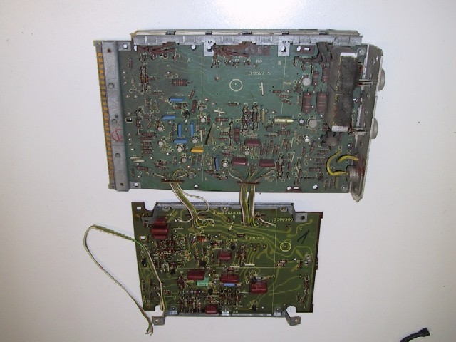
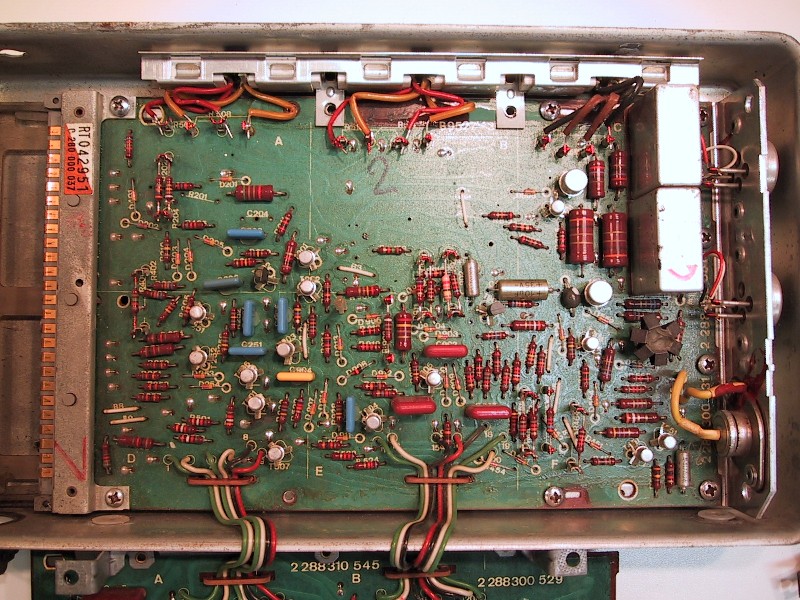
Main and Daughter Boards (0 280 000 037 ECU)
Main Board - This board has all the circuits on sheets 1 and 2 of the schematics below. D502 is the large diode on the heat sink on the right. The two germanium (AUY21) power transistors for the injector driver stage are also on the heat sink on the right. The power resistors are in the heat sink pack on the top (and are bonded to the ECU case for thermal transfer). According to Bosch, this main board is essentially the same for all D-Jetronic applications. Note the relatively empty area in the middle of the upper half of the board. On earlier ECU's (e.g. 0 280 000 015), this area was for the over-run shut-off circuit, which was removed on the 0 280 000 037, 0 280 000 043, and 0 280 000 044 ECU's. A more advanced version of the circuit returned on the 0 280 000 052 ECU's, used on the '75-'76 2.0L motors.
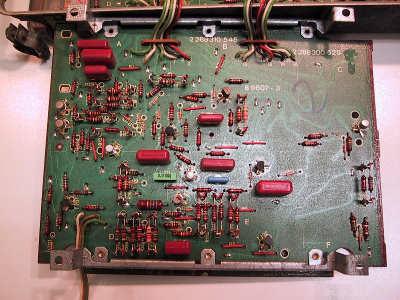
Daughter Board - This board has all of the circuits on sheet 3 of the schematics below. The 3-wire cable in the lower left is for the idle mixture adjustment potentiometer. Early ECU's (e.g. 0 280 000 015) lacked this control and used a different, smaller board design. According to Bosch, circuits on the daughter board are specific for each engine application. See the list of circuits on sheet 3 below for more information.
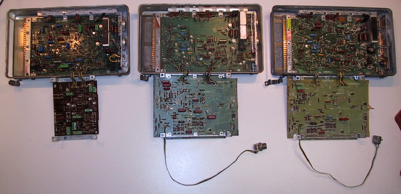
Below is a photo of three ECU's for comparison. From the left to the right: 0 280 000 015, 0 280 000 037, and 0 280 000 052.
A block diagram of the ECU can be found on page 0.1 - 1/8 of the Porsche 914 Factory Workshop Manual vol. 2, "Fuel System". While instructive, it does not accurately reflect the organization and components of the ECU. The diagram below is in the same spirit as the factory diagram, but was derived from review of the ECU schematics:
Below is a short description of each ECU block:
The TL controls which injector group is active, and signals the beginning of each injection cycle to the PL. The two switches in the TC are de-bounced and connected to the inputs of a flip-flop, creating square wave outputs from T251 and T252 that are 180 degrees out-of-phase. Each square wave output goes to an edge detector and the input NOR gate of the injector drivers (IL).
The edge detector is a differentiator circuit with a normal output of about +2 V. When a leading edge of the input square wave is detected, the differentiator generates a short negative-going pulse of about -12V. Pulses from both edge detectors are combined and are sent to the pressure-sensing loop circuit (PL). Each pulse is the starting signal for an injection pulse.
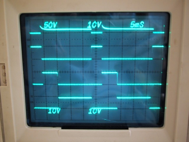
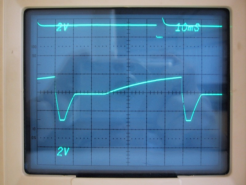
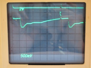
The traces in the oscilloscope photo below are (from top to bottom):
The PL creates a synchronized basic injection pulse, with the duration primarily controlled by the MPS. The heart of this circuit is the transistor pair T201 and T202. The basic injection pulse appears at the collector output of T202.
T201 is normally on, turning T202 off. With T202 off, its collector output is +12V. The negative-going pulses from the TL edge detectors turn T201 off, turning T202 on, which drives its collector output to zero volts. This causes a current to flow through L1 and the diode-resistor network (R401, R402 {if present}, R403, R405, D401, and TC1), inducing a negative voltage across L2. The time constant of the current decay is proportional to L1 * Re, where Re is the effective resistance value of the diode-resistor network. Since the inductances of L1 and L2 are dependent on the MPS armature position, the induced negative voltage on L2 is dependent on the manifold pressure (see my MPS document for a description of how the MPS works).
The negative voltage across L2 holds T201 off (keeps it turned off) through D202. As the current through L2 decays, the induced negative voltage decays, eventually to the point (starting at +0.7V) where T201 turns back on, turning T202 off, and completing the basic injection pulse. Bias voltage supplied from the SC and IM affects the basic injection pulse duration by shifting the voltage decay curve across L2. The more negative the bias voltage from the SC and IM, the longer the hold-off period and the longer the duration of the basic injection pulse.
"Luau_BoB" has graciously provided the following diagrams to better understand the effect of the SC and IM bias voltage on the pulse duration:
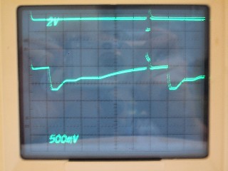
The traces in the oscilloscope photo below are (from top to bottom):
Note that since the resistance of TS1 is a component of Re, the time constant value is a function of the intake air temperature. From reading the resistors on a scrap ECU, I found the following resistance values: R401 = 1.5 K ohms, R403 = 510 ohms, and R405 = 1.5 K ohms. Ignoring the diode drop of D401, and using the nominal value of TS1 at 68 deg. F of 300 ohms, I calculate that Re = 395 ohms. If TS1 is open (disconnected), then Re = 436 ohms, about a 10% increase. If TS1 is shorted, Re = 381 ohms. Higher values of Re increase the time constant and richen the mixture. A common mechanic's trick is to disconnect the TS1 sensor on an older motor, increasing the injection pulse time by about 10% for a richer mixture. Older motors tend to have vacuum leaks and lower intake manifold vacuum (due to wear) than a new motor, so this trick often helps performance.
The OS circuit prevents injection during over-run to reduce emissions. When the throttle is fully closed, the idle switch is activated, grounding terminal "B" in the over-run shutoff circuit. This ground is one of the inputs to the base of T807, along with the output of a low-pass filter circuit that uses the basic injection pulse from the PL as an input. When the engine speed is above a threshold level (>2000 rpm?) and the throttle is fully closed, T807 is turned off, forcing T301 on, which inhibits injection. When the engine speed drops below the threshold, or if the throttle is opened, T807 is turned on, and the state of T301 is now determined by the basic injection pulse.
Note that this circuit is not present on all 914 ECU's. Below is an incomplete list of those ECU's with and without the OS circuit:
OS Circuit Present: 0 280 000 015, 0 280 000 052
OS Circuit Missing: 0 280 000 037, 0 280 000 043, 0 280 000 044
The IL combines multiple injection signals to create the final injection pulse. The T507 NOR gate enables injection when it receives a high signal from either inverter T301 (when the basic injection pulse from the pressure sensing loop goes low), the AE pulse output, or from the inverted output of the PWM.
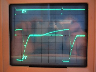
The traces in the oscilloscope photo below are (starting from the top):
The SL routes the final injection pulse to the appropriate injector group. The SL uses two NOR gates that each take the final injection pulse from the IL as one input. The other input of each NOR gate is from the two TL flip-flop outputs, which are square waves that are 180 degrees out-of-phase. When both the flip-flop output and the output of the IL are low, D1 or D2 are activated and the injectors are opened for the duration of the injection pulse. Because the inputs to the NOR gates are 180 degrees out-of-phase, only one injector group can fire for each injection pulse from T507.
D1 & D2 provide the appropriate current and voltage to drive the inductive load of the fuel injectors. Each driver uses two power transistors and load resistors to provide the proper voltage output to the injectors. Accounting for the 0.7 V drop across D502, and assuming a system voltage of 13.6 V when the car is running, 12.9 V is present at the emitters of the final driver transistors. Stefan von Allmen pointed out to me that these driver transistors are germanium devices, not silicon. Therefore, when the driver transistor turns on, there is an additional 0.2 V drop across the junction, so the effective supply voltage to the injectors is 12.7 V through a 6 ohm load resistor (Rload, a 5 W ceramic power resistor, bonded to the case of the ECU to act as a heat sink).
To understand the voltage waveform that appears across the injector, the injector is modeled as a series combination of inductance (Linj) and resistance (Rinj). Note that this is an approximate model only, because the injector is actually an electromechanical device, a solenoid. The characteristics of a solenoid are different than a simple inductor due to the electromechanical interaction of the moving armature and the coil inductance. Modeling the injector as a simple inductor, however, will be sufficient to describe the basic behavior.
The nominal specification value of Rinj is 2.4 ohms. Measurements I've taken on one of my injectors show Linj to be 3.77 mH and Rinj 2.69 ohms. When the driver transistor turns on and current begins to flow through the injector, a magnetic field begins to build in the coil and starts to pull the injector open. Due to the energy required to develop the magnetic field, the inductive reactance (XL - the effective resistance of the inductor to a time-varying signal, measured in ohms) is initially very large. Because XL is initially the largest resistance in the series path of circuit elements (Rload, Rinj, and XLinj), almost all of the voltage is dropped across the injector - that's why right after the injector turns on you see +12.7 V across it.
The rate the magnetic field builds is governed by the time constant, t = Linj / R, where R = Rinj. Therefore, t = 0.00377 / 2.69 = 1.40 msec. As the field builds, XL decreases and less voltage is dropped across the injector - that's why the voltage in the waveform below decays from the peak of +12.7 V. It takes about 2.5 * t for the decay to be complete, about 3.5 msec. Note that this means that for injection pulses shorter than this duration, the magnetic field is still decaying when the injector is turned off. Once the magnetic field is at steady-state, the voltage drop across the inductor is due solely to I * Rinj, where I is the steady-state current. If you use the nominal spec value of R = 2.4 ohms and an assumed battery voltage of +12 V, you would get a sustained voltage drop across the injector of 3 V. When the car is running, the actual system voltage is more like 13.6 V. Accounting for the higher measured injector resistance over the specification value and using the system voltage of 13. 6 V, the actual measured sustained voltage is 4 to 5 V. Note that the calculated drive voltage corresponds exactly with data given for the flow rates of the injectors, which states that the tests were performed at 3 V (data courtesy of Roland Kunz).
At the end of the injection period, the driver transistor turns off, which rapidly changes the current drive to the injector to zero. The rapid collapse of the magnetic field in the coil now has an opposite effect - it induces a high negative voltage across the inductor. The mathematical expression of this voltage is VL = Linj * dI/dt , where dI/dt is the time derivative of current through the inductor. The net effect is that you get a large negative spike of voltage after the injector turns off. I have measured a peak of -27 V, decaying in about 1 msec to zero volts. The inductive voltage spike (and resultant current) is limited by the series combination of a 6.8 mF capacitor and load resistor in parallel with the injector. Note that since D-Jetronic is a grouped injection system, a paired set of injectors experience all of the events described above simultaneously. When the injectors turn off, the inductive voltage spike of both injectors is limited by the 6.8 mF capacitor and load resistor.
Note that this analysis ignores the high impedance path from the final driver transistor emitters through R510 (820 ohms) and D501, which is negligible in comparison with the low-impedance path through the injectors.
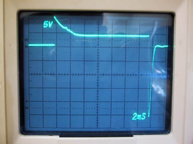
Below is a photograph of an injector waveform I measured on my car, ground is 2 divisions down from the top:
Below is a pSpice schematic I used to simulate the behavior of this circuit, with actual values I measured on each component from a 0 280 000 037 ECU that I have disassembled, and the injector values from one of the injectors in my car. All parameters were measured with a Wavetek LCR55 component analyzer. This analysis assumes a silicon driver transistor, with a 0.7V junction voltage, instead of the actual germanium device, which has a 0.2 V junction voltage, which would bring Vsupply to about 12.7 V. The effect of this difference is a very slight increase in the negative swing of voltage after the injector closes.
Below are the results of the simulation, measuring the voltage at the node indicated on the schematic. This node is the equivalent of measuring the voltage waveform at the injector.
The differences between the simulation and the measured waveform are attributable to the approximation of the injector solenoid by a simple inductor. Note that all of the basic characteristics of the waveform are the same as the measured waveform. The oscillations at the close of the injection cycle are due to the LCR oscillator circuit not being critically damped. This ringing is not present in the actual waveform as the solenoid's characteristics apparently are so as to provide additional damping. Note also that the initial decay starting at 0 s is more rapid than in the actual waveform due to the neglect of the mechanical work done by the solenoid. Lastly, note the good correlation between the maximum extent of the negative induced voltage when the injector closes with the actual waveform value of about -27 V.
The AE circuit provides immediate and delayed enrichment when the throttle is opened for acceleration. Throttle opening is signaled by the TPS through alternating ground signals from two inter-digitated traces that are each connected to the inputs of a flip-flop (see sheet 2 of the schematic for a drawing of the switch details). A drag switch in the TPS prevents these signals from being sent when the throttle is closing. The outputs of the flip-flop are sent to two edge detectors, whose outputs are combined and sent to pulse shaping and narrowing circuits. The pulse shaper provides immediate injection pulses to the IL. The width of these pulses is independent of engine speed and load, and from Kerfoot's schematic, they are about 1.5 ms in duration. An additional acceleration enrichment effect is created by sending the inverted, shaped, and narrowed pulses to the mixture enrichment circuit. The negative-going pulses pump up the voltage on capacitor C901, controlling and turning on T901, which acts as a current source. This current is sent to the the PWM, where it helps charge up the 0.68 F capacitor that defines the raw delayed pulse waveform for the mixture adjustment. After the pulses stop, C901 slowly discharges over about 2 to 3 seconds, and the acceleration enrichment effect goes away.
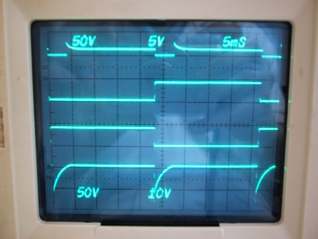
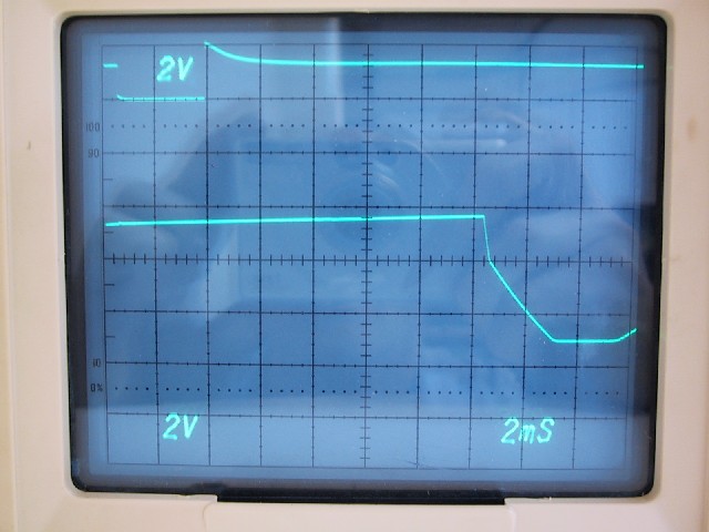
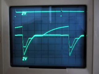
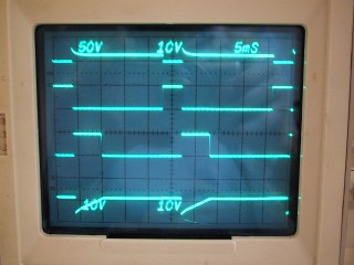
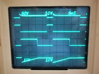
The traces in the oscilloscope photo below are (starting from the top down):
The bottom half of the screen is in storage mode. I switched on the accelerator pulses from the TPS, then turned it off. When on, the output from the PWM (trace 3) extended by about 1.0 ms. When I turned the TPS pulses off, trace 3 relaxed back to the original value, over a period of about 2 seconds and smearing the trace, demonstrating the "delayed" acceleration effect. Trace 4 shows the 1.5 ms pulses from the AE that are being simulated by the EFI 1401 tester. To avoid pulse width measurement jitter, the pulses are timed to occur during the basic injection pulse, thereby not contributing to the injection duration. However, in actual operation, these pulses occur asynchronously and do contribute to the injected quantity during acceleration.

The FPC operates the FPR during starting and normal running. The FPR is controlled by T552, which when on, provides ground to the FPR. When the key is turned to the "on" position, +12V is supplied to the ECU, and the FPR is activated for 1.5 seconds. At power-on, T101 is on and T102 is off because C101 has not charged to 1.4 V yet. While T102 is off C102 is charging and T103 is On. Eventually C101 charges and turns T102 on which pulses T103 to off via the discharge of C102. The pulse charges C551, turning the FPR on, then C551 discharges (taking about 1.5 sec), turning the FPR off. Turning the key to the "start" position sends the Start signal to the base of T552, activating the FPR. If the car starts, and the engine speed is greater than 100 rpm, pulses from the ES pump up capacitor C551, turning T551 and T552 on, activating the FPR . If the engine speed drops below 100 rpm, there is insufficient pumping to keep the voltage on C551 high enough to keep T551 on, shutting off the FPR.
The CTC adjusts the mixture for the engine temperature. The operation of the circuit is controlled by T451, which is operated in the linear region. T451 is part of a resistor-diode voltage divider circuit. The resistance across T451 in this circuit is controlled by the base drive. Ignoring start and idle conditions (CTC effects under these conditions are covered in ICM section), the drive is defined by the voltage divider of TS2 and R464 (assuming near zero base current). When the engine is cold, TS2 is about 2300 ohms, and the base voltage is about 7.7 V, driving T451 towards saturation, decreasing the voltage drop across the transistor. I did not do the circuit analysis of the resistor-diode voltage divider circuit, but Frank Kerfoot notes that the effect of this decreased voltage drop across T451 is to drive the output of the CTC to a higher voltage, increasing the multiplication effect in the PWM. Similarly, when the engine is hot, TS2 is only about 50 ohms, resulting in a base voltage of only 0.4 V, turning T451 nearly off, and increasing the voltage drop across the transistor. This drives the output of the CTC lower, decreasing the multiplication effect in the PWM.
What happens to the CTC output if TS2 is open or shorted? If TS2 is open, the base of T451 is effectively at +12V, driving T451 into saturation. This causes the output of the CTC to go to a maximum, which results in a very rich mixture, preventing the car from running after starting. If TS2 is shorted, the base of T451 is effectively grounded, and T451 is fully off. Under cold engine conditions, this results in a very lean mixture, lean enough to prevent the engine from running. For a hot engine, the effect is not as significant, and the engine may run, but will be lean.
I simulated the CTC with pSpice, using measured component values from a 0 280 000 037 and a 0 280 000 052 ECU that I have disassembled. T451 was simulated using a standard 2N2222 npn transistor model. The 037 and 052 component values are significantly different for some resistors in the CTC, and the 037 lacks the 270 ohm R471 present in the 052. The output voltage was modeled as a function of TS2 resistance, over a range for a 0 280 130 012 sensor that corresponds to a temperature span from 39 F to well above operating temperature. Results are shown below:
These results are very interesting. First, they point out that once TS2 drops below about 300 ohms on Vout for both the 037 and 052 ECU's, any subsequent decrease in resistance has little to no effect on Vout. They also show that there are significant differences in the warm-up characteristics of the two ECU's. The 052 is leaner during warm-up, but essentially the same once fully warmed-up. I do not have an 043 or 044 ECU that is disassembled to compare these results to, and the 015 ECU that I have has a completely different CTC circuit that I have yet to analyze.
In early 2010, I used my EFI bench setup to verify the pSpice simulation results. The correlation was excellent, the cut-off resistance of TS2 was around 330 to 350 ohms for the 037, 043/044, and 052 ECU's. I also verified that this cut-off behavior was independent of engine load and speed.
Below I've added traces that show the effect of the idle switch in the 052 ECU and the effect of adding ballast resistance to the 017 TS2 sensor with the 037 ECU.
The '73 2.0L motor used a different temperature sensor with a series 270 ohm ballast resistor. Note that if you compare values at equal temperatures instead of equal resistance (see the faint dashed lines on the graph), the values of Vout are nearly the same as for the case of the 052 ECU with the 0 280 130 012 temperature sensor. This is how Porsche was able to use the 037 ECU, which was intended for the 1.7L motor, with the 2.0L motor and get the proper warm-up characteristic. Below is a small table quantifying the comparison:
| Temperature | 052 ECU w/012 TS2 | 037 ECU w/017 TS2 | % difference |
| 39 F | 8.348 V | 8.039 V | -3.7% |
| 61 F | 6.945 V | 6.959 V | 0.2% |
| 210 F | 4.090 V | 4.249 V | +3.9% |
The 052 ECU has a circuit that switches in an additional 270 ohm ballast resistance when the idle switch is on. This provides additional enrichment when warming up at idle as compared to the '73 2.0L setup. I do not know if the '74 2.0L setup has this switchable idle ballast resistance.
Note that all of the variation displayed above demonstrates why it is so important to only set the CO at idle when the motor is fully warmed-up and is operating in the flat portion of the Vout curve. Otherwise, variations due to TS2 resistance as a function of head temperature will likely result in the wrong final mixture.
These data also have application for using ballast resistance for tuning. It has been a common practice to add ballast resistance to the TS2 sensor to increase the richness of the mixture to accommodate larger displacement and other modifications. The problem that the data above point out is that if you do this when the motor is fully warmed-up, the amount of ballast you need to add will need to be such that the combined resistance of the ballast and the TS2 sensor exceeds about 300 ohms. Since TS2 drops to as little as 50 ohms when the motor is hot (head temps of 300 F, for example), this means that the ballast will be more than 250 ohms. But because TS2 resistance increases rapidly as the engine temperature decreases, the proportional effect on Vout decreases. This means that for cold and cold-cold start conditions, the mixture will not be rich enough for a large-displacement motor for good characteristics. As a result, using ballast resistance to increase the overall mixture will likely lead to drivability problems.
Using ballast resistance to improve warm-up characteristics, however, has some good potential. If you are experiencing problems with a lean mixture during warm-up, a modest amount of ballast resistance (e.g. 50 ohms) will produce a richer mixture, but will not affect the mixture when the motor is fully warmed up. This permits, within a range, the independent adjustment of warm-up mixture, idle mixture, and hot mixture. An alternative approach to improving the warm-up by enriching the mixture is to use a steel spacer or standoff between TS2 and the head. This was the solution that VW implemented on the 2.0L Bus engine. The idea is that the thermal response of the sensor with regard to head temperature changes is delayed due to the steel standoff, leading to a richer mixture. Once fully warmed up, the spacer approaches the head temperature, and also damps out fluctuations due to rapid swings in head temperature. Such spacers are NLA and have to be fabricated (see the Q&A section below for details). I am using a spacer on my 2.0L engine, it completely eliminated problems I had with a lean start-up mixture and enabled me to remove any ballast resistance from the TS2 circuit.
Note also that using head temperature to sense the cylinder combustion chamber temperature of an air-cooled motor has significant drawbacks. The head is made of aluminum, the cylinder is made of cast iron, which retains heat for much longer than aluminum. Additionally, head temperature varies widely due to its dependency on load. The net result is that mixture correction as determined by head temperature can lead to lean or rich mixtures, depending on the situation. For example, if an air-cooled engine is warmed up, then shut down for 15-20 minutes, the head cools dramatically while the cylinder remains quite hot, causing the ECU to provide a very rich mixture on re-starting. This is a classic problem with 2.0L 914 engines.
The graph below demonstrates the effect of small and large amounts of ballast resistance on the characteristics. Regions corresponding to the various temperature conditions are displayed.
The ES creates an engine speed signal used by the FPC and the SC. The input to the ES is the basic injection pulse from the PL. T101 and associated circuitry act as an edge detector for the trailing edge of the injection pulse. The output of the edge detector is shaped by T102 into a 0.5 ms pulse (this point is also coupled to the PWM, apparently for voltage clamping) and to T103, where the output is stretched and inverted to form the engine speed signal. This signal is used by the FPC to detect if the engine is running faster than 100 rpm.
The ES output is fed to the SC circuit. The function of this circuit is to correct the mixture for the volumetric efficiency (Ve) curve of the engine. "Luau_BoB" saw my pitiful first draft on this section and took it upon himself to provide the excellent analysis I have paraphrased here, with modified versions of his diagrams to match the nomenclature of this document.
Volumetric efficiency (Ve) is the ratio of the actual volume of air taken in by a cylinder divided by the cylinder volume. The maximum Ve is mostly determined by the design of the intake system (2 vs. 4 valve, valve sizes, intake runner design, throttle body design, air filter, etc.), and the engine speed at which the maximum Ve occurs is mostly determined by valve timing and by intake runner design. Typical max Ve for an engine with a overhead 2-valve configuration is about 75 to 80%. A generalized Ve curve for an engine is shown below:
Here are two good basic references on Ve:
http://www.tpub.com/engine1/en1-105.htm
http://www.ponycarburetors.com/calculating_cfm.htm
A good reference that shows how to measure the Ve of an engine is:
To maintain a constant air/fuel ratio, the fuel quantity must take into account the Ve at a specific engine speed. The SC circuit is used to realize this effect.
The following diagrams are used to describe the SC operation:
In this simplified model, the SC is replaced by a generalized waveform generator (Wf), and the PL is represented by T201, T202, and the MPS. As the Wf bias voltage changes, the threshold for turn-on of T201 changes, which in turn, changes the basic injection pulse duration. See the diagram above in the PL analysis to see how this works.
The effect of the Wf bias voltage on the basic injection pulse generated by T202 is shown below:
In the example above, the actual Wf output is modeled by a hypothetical linear voltage decay, V(t) = -k * t + b , where k is the slope and b is the offset voltage. Note that the value of V(P) determines the turn-on voltage for T201, which determines the basic injection pulse duration. In the case of this hypothetical Wf, then as engine speed increases, P decreases, and V(P) increases. As shown in the diagram above, as V(P) increases, T becomes shorter.
A model of the waveform generators in the SC of the 0 280 000 052 ECU is shown below:
The output of each of the Wfm generators are "OR'ed" together, which results in an output signal that is the maximum voltage of all of the waveforms at a given time. Why four Wfm generators? The reasons will become in a moment. The sketch below is a composite of all of the Wfm generators "OR'ed" together, to show how each contributes to the complete waveform:
From the sheet 3 of the schematic, note that the Wfm 1, 2, and 3 generators each have selected components (resistors) , picked to match the specific Ve curve of the engine application the ECU was designed for. The Wfm4 generator is a simple voltage divider that generates the 4.8V output. The output of the Wfm's are buffered by T107 (emitter-follower). The buffered output signal is combined with the output of the IM and sent to the PL, where it sets the threshold for the turn-off of T201. Note that for non-idle conditions, the output of the SC controls the T201 threshold, whereas at idle conditions, the output of the IM dominates.
The final waveform at the base of T107 in the diagram above is from Kerfoot's schematic. Randy Montellato has recently measured this characteristic on his ECU. See below:
The characteristic is similar to Kerfoot's measurement of the base of T107, noted on sheet 3, and is also similar to the characteristic of the composite waveform diagram above. The influence of each waveform generator's can be identified.
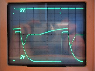
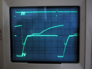
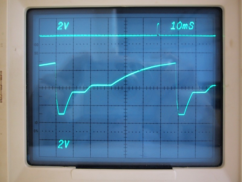
Below is a series of scope photos I took that show the behavior of the waveform generators with respect to the injection pulse. The ECU under test is a 0 280 000 052 and the MPS is a 0 280 000 049 (NOS unit from Gary Helbig). The simulated engine speed is 950 rpm to show the full characteristic. The overall Wfm characteristic was measured at the base of T107.
At the top is the basic injection pulse (ti), measured at the output of the PL. The influence of two of the waveform generators can be thought of as DC levels connected by smooth transitions. For this case:
Wfm1 = 7.8 V
Wfm4 = 5.0 V
The other two waveform generators affect the beginning and end of the overall waveform. Wfm2 defines the transition at 10 ms from the previous waveform down to the Wfm4 level. Wfm3 defines the continuously-rising characteristic from about 40 ms to nearly 80 ms.
The plot below uses a delayed trigger to precisely position the trailing edge of the injection pulse to measure the the duration between this edge and the onset of the Wfm waveform.
With this greater precision, the interval is actually 11 ms, corresponding to an engine speed of 5455 rpm. This is significant because the redline of the 1.7 and 2.0L motors is 5850 rpm, which means that just before redline, the speed correction reaches the flat portion of the curve above, between 11 ms and 10.25 ms.
Examination of the SC schematic shows that the DC levels for Wfm1 and Wfm4 are set by voltage dividers in each of the Wfm generators. The capacitors and other circuit characteristics determine the waveform shape. It appears that for the most part, Bosch adjusted the DC levels by changing the voltage divider elements to match the curve for each engine application.
The trailing edge of the injection pulse indicates the time position where the level of voltage at the base of T107 that was used by the PL to set the turn-on voltage of T201, buffered through T107. As the engine speed increases, the period between injection pulses ti decreases, and the voltage at the base of T107 at the trailing edge of ti moves leftwards through the overall Wfm characteristic. In the case above, the voltage level at T107 at the trailing edge is being determined by the Wfm3 generator. As engine speed increases, the Wfm1, then Wfm4, then finally Wfm2 generators will determine the PL T201 turn-on voltage.
Below are scope photos that show the influence of each Wfm generator on the overall characteristic. Note that each Wfm generator's characteristic is shifted slightly positive due to the diode voltage drop when forward biased:
| Wfm1 | Wfm2 | |
 |
 |
|
| Wfm3 | Wfm4 | |
 |
 |
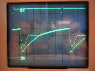
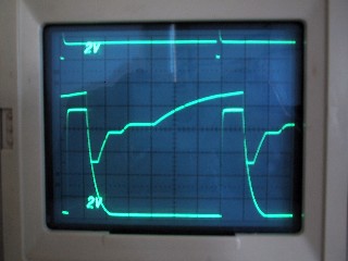
Below is a similar set of scope pictures for a 0 280 000 037 ECU, taken under identical conditions to the 052 ECU above. This ECU has an additional Wfm (Wfm5) that adds a "step" between 27 to 40 ms.
Below are scope photos that show the influence of each Wfm generator on the overall characteristic. Note that each Wfm generator's characteristic is shifted slightly positive due to the diode voltage drop when forward biased:
| Wfm1 | Wfm2 | |
 |
 |
|
| Wfm3 | Wfm4 | |
 |
 |
|
| Wfm5 | ||
 |
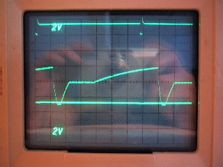
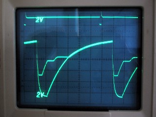
Below is a scope photo of the overall SC waveform from a 0 280 000 015 ECU, used on early 1.7L's. Conditions are the same as for the two ECU's above. There are five Wfm's, similar to the 0 280 000 037 ECU.
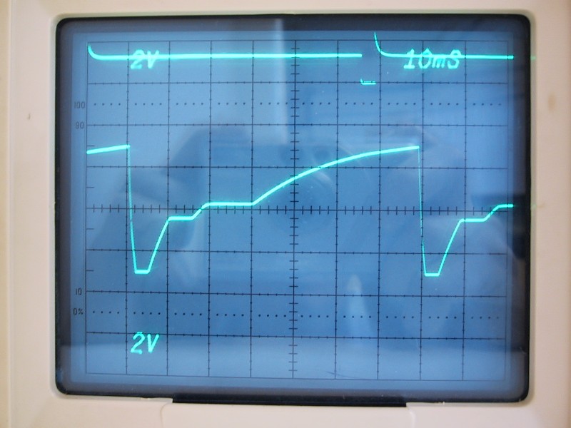
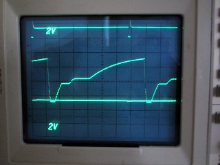
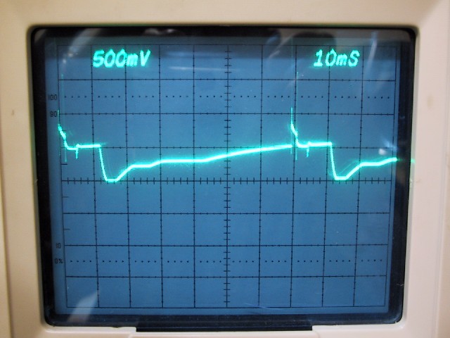
Below is a measurement taken at pin 10 of the edge connector on a 0 280 000 044 ECU, showing the level-shifted, combined output of the SC and IM circuits. Note that this characteristic can be fairly easily measured with an oscilloscope on any D-Jetronic system by probing pin 10 of the MPS. Ground at the bottom of the screen. Note the effect of the triggering of the loop circuit is visible at about 70 mS. The control voltage ranges between 2.0 and 2.5 V. It is also apparent that this ECU uses 5 Wfm's, as the waveform is similar to the 015 and 037 ECU's.
To understand the effect on the injection pulse duration at a specific engine speed, first note that lower values of bias voltages affect the PL circuit to extend the injection period (see the PL section for a description of this behavior), increasing Tinj. On sheet 3, the opposite behavior is noted, so this observation is in disagreement with Kerfoot's notes which appear to be in error. Next, since the bottom axis is time, engine speed is proportional to the reciprocal of time. Therefore, you need to invert and flip the characteristic as shown below:
The characteristic above reflects the Ve behavior of the specific engine application. Now, the need for four waveform generators is clear. Wfm3 sets the speed correction at low-rpm's near idle. Wfm1 sets the speed correction at medium-rpm, approaching the Ve peak. Wfm4 sets the speed correction for the high-rpm Ve peak. Finally, Wfm2 sets the speed correction between the high-rpm Ve roll-off as redline is approached. By varying the selected resistors and capacitors in the Wfm circuits, a wide range of Ve curves can be accommodated with the SC circuit.
Below is a plot I created from analysis of the overall waveforms for both the 037 and 052 ECU's above that corresponds to the model plot of effect on injection time as a function of engine speed. The y-axis was inverted by re-referencing it to the system voltage.
This plot shows the speed correction effects of both ECU's very clearly.
Randy Montellato also characterized the effect of the SC on the injection pulse width by monitoring the pulse width on a bench setup of the D-Jetronic system as a function of engine speed at constant intake manifold pressure. A chart of his results is shown below:
The results shown compare favorably with the inverted and flipped Wfm output, especially under full-load (0 in. Hg) conditions. Note that it appears that the long injection durations at low RPM implied by the Wfm bias characteristic apparently are at engine speeds well below the idle point, where the bias value is controlled by the IM instead of the SC.
I recently obtained a D-Jetronic tester that enables the simulation of engine speed and sensor settings. I've duplicated the characteristics that Randy took for three operating conditions: at operating temperature (~100 C), cold start (20 C), and cold-cold start (-10 C). Missing data on the cold and cold-cold graphs are due to tester limitations.
My cold start data is very similar to Randy's. The speed-density nature of the D-Jetronic system is clear from this data. Note the dramatic increase in injection duration with cold temperatures. From what I've been able to find out, this relationship of richer mixture to colder temperatures is empirically derived for each motor, due to variations in the intake design and motor heating characteristics.
Recently, I obtained a copy of the original Bosch papers (see References) that describe the development of the D-Jetronic system. Figure 2 from the H. Scholl paper is essentially identical in shape and nature to both Randy's and my graphs above:
The text associated with this graph states that this is the characteristic diagram of the fuel requirement for one cylinder of a six-cylinder engine, measured on an engine test stand.
"Vollast" = full load, corresponding to the "0 in. Hg" curve in Randy's and my graphs. Manifold pressures here are measured in Torr, an absolute scale as opposed to a gauge scale like inches of Hg. Assuming 760 Torr = 0 in. Hg, the manifold pressures levels map as follows:
0 in. Hg = 760 Torr
5 in. Hg = 633 Torr
10 in. Hg = 506 Torr
15 in. Hg = 380 Torr
20 in. Hg = 250 Torr
Randy's readings at 20 in. Hg are considerably lower that the lowest reading on the Bosch graph, and are also near the limits of movement of the armature core of the MPS. Bosch went further in detail on their graph of full-load, noting the small vacuum that is pulled in the plenum due to the pumping restrictions of the throttle body and intake system, growing with increasing engine speed to a 20 Torr drop at maximum engine speed. Since the cylinder volume of the six-cylinder engine used in the diagram from the Scholl paper is unknown, and is likely smaller than the cylinder volume of the 2.0L four-cylinder motor that Randy and I used for our measurements, leading to the absolute difference in the injection time between the graphs at any specific manifold pressure.
The PWM stretches the basic injection pulse width to correct the mixture for the effects of engine temperature (CTC) and linked effects, starting enrichment (ICM), and the delayed accelerator pump action (AE). See the scope photo above for an example of the output of the PWM. The basic injection pulse from the PL is fed to the base of T302. The collector output of T302 charges the 0.68 mfd capacitor, which is also charged by the current source from the AE that provides the delayed accelerator enrichment effect. The collector output of T303 sets the voltage on the other side of the capacitor, also affecting the charging rate of the capacitor. The drive on T303 is set by the output of the CTC, and the emitter level of T303 is set by the resistor-diode network, and also by a start signal effect from T651 (see the ICM description below). Diode D302 is then used to shape the sawtooth signal output into more of a square wave. This shaped signal is then sent to the IL to multiply the effect of the basic injection pulse from the PL.
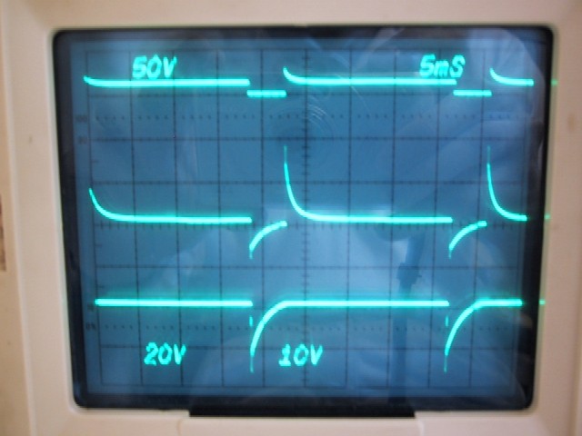
The traces in the oscilloscope photos below are (starting down from the top):
The effect of changing the value of the TS2 on the PWM output is demonstrated.
 |
 |
| Engine at operating temperature (~100 C) | Cold engine (~20 C) |
The ICM provides cold-start enrichment clamping, idle mixture enrichment, and starting mixture enrichment to the PWM.
The IM sets the mixture (adjustable with IA) during idle operation. The output of the IM is combined with the output of the SC to control the voltage threshold in the PL for turn-off of T201. When the throttle is open, the IM appears as an open circuit and the SC controls the PL threshold. Note that the IM is effective ONLY when the IS on the TPS is closed!! Adjustment of the IA has no effect on mixture when the throttle is open.
T701 acts as a current source through R705 and the 5 K adjustment potentiometer (IA). The voltage divider implemented with the potentiometer sets the PL threshold level. The effect of adjusting the IA is to shift the entire SC curve on the voltage axis. The two scope photos below (sorry for the poor quality) show the effect of the IA potentiometer position (measured at point 15 on sheet 3 of the schematic) on the combined IM+SC output for a 0 280 000 037 ECU under test at idle conditions. Total voltage shift range is about -0.6 V going from fully counter-clockwise to fully clockwise. Note that this range of adjustment is comparable to the entire range of voltage shift over the complete SC curve (about 0.7V), indicating that the IM is capable of a wide range of mixture adjustment at idle.
 |
 |
| IA Fully Counter-Clockwise (Lean) | IA Fully Clockwise (Rich) |
On most ECU's with an IM knob, there is a small mark in the plastic surround of the knob that was put there at the factory. This mark identifies the balance point where the IM adjustment has no effect on the level of the output of the SC circuit. For a new motor in good adjustment, this point produces a CO level very close to the factory specification.
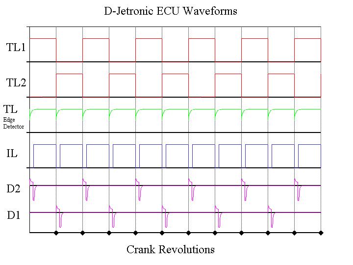
TL1 and TL2 are the outputs of the flip-flop in the TL circuit. The edge detector generates a short negative-going pulse (down from +12V) on each rising edge from either TL1 or TL2. This signal goes to the PL, which generates the basic injection pulse, which is modified by the IL for effects from the PWM and the AE (additional AE pulses are not shown here). The IL signal and the TL1 and TL2 signals are inputs to the NOR gates for D1 and D2. When both inputs are low, the injector group for D1 or D2 will be energized. Note that the injector groups fire every other crank revolution.
The VW1218 also does comprehensive testing of the FI sensors, including the MPS. Note that the Bosch EFAW tester also available for rental from Pelican Parts only does static testing of the TS1 and TS2 sensors, system voltages, MPS resistances, and does a qualitative test of the trigger contact points and MPS function.
In lieu of using the VW1218, a suspect ECU can be swapped with a
new/rebuilt ECU. Note that there is also an aftermarket D-Jetronic tester
that was available about 20 years ago called the "MPC Analyzer"
- again, see my
D-Jetronic Testers web pages for a description.
A few shops still have this tester, which is an advanced tool for
evaluating the ECU operation. It can also be used to adjust
the MPS to factory settings. John Larson on Rennlist has one of these
testers at his shop in Central California, please contact him for further
information.
Special thanks to Jim Thoursen, Dave Darling, Roland Kunz, and others on Rennlist who have assisted me with this analysis. Big thanks to Frank Kerfoot for the excellent work he did on the schematic and his assistance with the analysis. Big thanks to "Luau_BoB", who took it upon himself to analyze the SC circuit, and improve the description of how the SC and IM bias voltage affects the basic injection pulse duration. Thanks also to Randy Montellato for his measurements of the effects of engine speed on injection duration. Thanks also to Jeff Bowlsby for his comments and assistance with some of the measurements. Thanks to Stefan von Allmen for his contributions to the injector driver circuit analysis.